머신러닝 공부하기 2탄!
파이썬 라이브러리를 활용한 머신러닝 책을 참고하여 작성하였다.
2) 지도학습
- 입력과 출력 샘플 데이터가 있고, 주어진 입력으로부터 출력을 예측하고자 할 때 사용
- 입력/출력 샘플 데이터, 즉 훈련 세트로부터 머신러닝 모델을 만든다.
- 목표 : 이전에 본 적 없는 새로운 데이터에 대해 정확한 출력을 예측하는 것
2-1) 분류와 회귀
- 분류(classification) : 미리 정의된, 가능성 있는 여러 클래스 레이블 중 하나를 예측하는 것
- 이진 분류 : 두 개의 클래스로 분류 (Y/N)
- 다중 분류 : 셋 이상의 클래스로 분류
- 회귀(regression) : 연속적인 숫자, 또는 프로그래밍 용어로 말하면 부동소수점수(실수)를 예측하는 것
- 출력 값에 연속성이 있는지 = 예상 출력 값 사이에 연속성이 있다면 회귀 문제
2-2) 일반화, 과대적합, 과소적합
- 일반화(generalization) : 모델이 처음 보는 데이터에 대해 정확하게 예측할 수 있을 때 이를 훈련 셋 에서 테스트 셋으로 일반화 되었다고 한다.
- 그래서 모델을 만들 때에는 가능한 정확하게 일반화되도록 해야한다.
- 보통 훈련 셋에 대해 정확히 예측하도록 모델을 구축.
- 아주 복잡한 모델을 만든다면 훈련셋에만 정확한 모델이 되어버릴수도 있다.(오버피팅)
- 오버피팅(overfitting) : 가진 정보를 모두 사용해서 너무 복잡한 모델을 만드는 것
- 모델이 훈련셋의 샘플에 너무 가깝게 맞춰져서 새로운 데이터에 일반화되기 어려울 때 발생
- 언더피팅(underfitting) : 너무 간단한 모델이 선택되는 것
- 그렇게 되면 데이터의 다양성을 잡아내지 못할 것이고 훈련셋에도 맞지 않는다.
- 오버피팅(overfitting) : 가진 정보를 모두 사용해서 너무 복잡한 모델을 만드는 것
- 모델을 복잡하게 할수록 훈련 데이터에 대해서는 정확히 예측할 수 있다. 하지만 너무 복잡해지면 훈련셋에 각 데이터 포인트에 민감해져 새로운 데이터에 일반화되지 못한다.
- 우리가 찾으려는 모델은 일반화 성능이 최대가 되는 최적점에 있는 모델
모델 복잡도와 데이터셋 크기의 관계
- 모델 복잡도는 훈련 데이터셋에 담긴 입력데이터의 다양성과 연관이 깊다. 데이터셋에 다양한 데이터 포인트가 많을수록 과대적합 없이 더 복잡한 모델을 만들 수 있다.
2-3) 지도학습 알고리즘
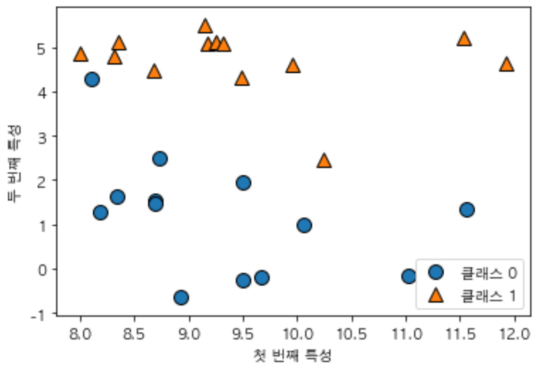
forge 데이터 셋 : 인위적으로 만든 이진분류 데이터셋
- 이 데이터셋의 모든 데이터 포인트를 산점도로 그린다.
- x축은 첫번째 특성, y축은 두번째 특성
- 점 하나가 데이터 포인트를 나타낸다.
- 점의 색과 모양은 데이터 포인트가 속한 클래스를 나타낸다.
import pandas as pd
import mglearn
import numpy as np
import matplotlib.pyplot as plt
from IPython.display import display
import matplotlib
matplotlib.rc('font', family='AppleGothic')

plt.rcParams['axes.unicode_minus'] = False
X, y = mglearn.datasets.make_forge()

mglearn.discrete_scatter(X[:,0], X[:,1], y)
plt.legend(['클래스 0', '클래스 1'], loc=4)
plt.xlabel('첫 번째 특성')
plt.ylabel('두 번째 특성')
print("X.shape: {}".format(X.shape))
X.shape: (26, 2)
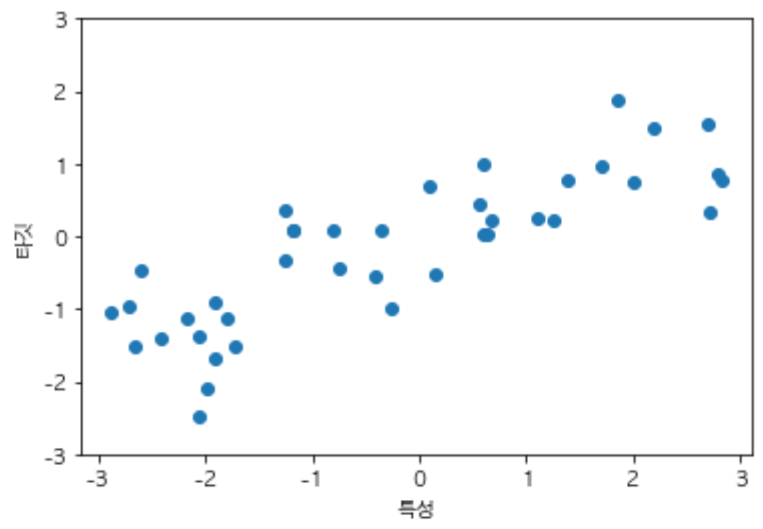
Wave 데이터셋
- 입력 특성 하나와 모델링할 타깃 변수를 가진다.
- 아래의 그림은 특성을 x축에 두고, 회귀의 타깃(출력)을 y축에 두었다.
X, y = mglearn.datasets.make_wave(n_samples=40)
plt.plot(X,y,'o')
plt.ylim(-3,3)
plt.xlabel('특성')
plt.ylabel('타깃')
Text(0, 0.5, '타깃')
- 특성이 적은 데이터셋(저차원 데이터셋)에서 얻은 직관이 특성이 많은 데이터셋(고차원 데이터셋)에서 그대로 유지되지 않을 수 있다.
- 알고리즘을 배울때 저차원 데이터셋을 사용하는 것이 좋다.
scikit-learn에 들어있는 실제 데이터셋 사용
- 1) 위스콘신 유방암 데이터셋(Wisconsin Breast Cancer) : 유방암 종양의 임상 데이터 기록
- 양성(해롭지 않은 종양)과 악성(암 종양)으로 레이블링 되어있고, 조직 데이터 기반으로 종양이 악성인지를 예측할 수 있도록 학습하는 것이 과제.
- 2) 보스턴 주택가격(Boston Housing)
- 범죄율, 찰스강 인접도, 고속도로 접근성 등의 정보를 이용해 1970년대 보스턴 주변의 주택 평균 가격 예측
Wisconsin Breast Cancer
from sklearn.datasets import load_breast_cancer
cancer = load_breast_cancer()
print("cancer,keys(): \n{}".format(cancer.keys()))
cancer,keys():
dict_keys(['data', 'target', 'target_names', 'DESCR', 'feature_names', 'filename'])
- 데이터에 대한 자세한 정보 확인
print(cancer['DESCR'])
.. _breast_cancer_dataset:

Breast cancer wisconsin (diagnostic) dataset
--------------------------------------------

**Data Set Characteristics:**

    :Number of Instances: 569

    :Number of Attributes: 30 numeric, predictive attributes and the class

    :Attribute Information:
        - radius (mean of distances from center to points on the perimeter)
        - texture (standard deviation of gray-scale values)
        - perimeter
        - area
        - smoothness (local variation in radius lengths)
        - compactness (perimeter^2 / area - 1.0)
        - concavity (severity of concave portions of the contour)
        - concave points (number of concave portions of the contour)
        - symmetry
        - fractal dimension ("coastline approximation" - 1)

        The mean, standard error, and "worst" or largest (mean of the three
        largest values) of these features were computed for each image,
        resulting in 30 features.  For instance, field 3 is Mean Radius, field
        13 is Radius SE, field 23 is Worst Radius.

        - class:
                - WDBC-Malignant
                - WDBC-Benign

    :Summary Statistics:

    ===================================== ====== ======
                                           Min    Max
    ===================================== ====== ======
    radius (mean):                        6.981  28.11
    texture (mean):                       9.71   39.28
    perimeter (mean):                     43.79  188.5
    area (mean):                          143.5  2501.0
    smoothness (mean):                    0.053  0.163
    compactness (mean):                   0.019  0.345
    concavity (mean):                     0.0    0.427
    concave points (mean):                0.0    0.201
    symmetry (mean):                      0.106  0.304
    fractal dimension (mean):             0.05   0.097
    radius (standard error):              0.112  2.873
    texture (standard error):             0.36   4.885
    perimeter (standard error):           0.757  21.98
    area (standard error):                6.802  542.2
    smoothness (standard error):          0.002  0.031
    compactness (standard error):         0.002  0.135
    concavity (standard error):           0.0    0.396
    concave points (standard error):      0.0    0.053
    symmetry (standard error):            0.008  0.079
    fractal dimension (standard error):   0.001  0.03
    radius (worst):                       7.93   36.04
    texture (worst):                      12.02  49.54
    perimeter (worst):                    50.41  251.2
    area (worst):                         185.2  4254.0
    smoothness (worst):                   0.071  0.223
    compactness (worst):                  0.027  1.058
    concavity (worst):                    0.0    1.252
    concave points (worst):               0.0    0.291
    symmetry (worst):                     0.156  0.664
    fractal dimension (worst):            0.055  0.208
    ===================================== ====== ======

    :Missing Attribute Values: None

    :Class Distribution: 212 - Malignant, 357 - Benign

    :Creator:  Dr. William H. Wolberg, W. Nick Street, Olvi L. Mangasarian

    :Donor: Nick Street

    :Date: November, 1995

This is a copy of UCI ML Breast Cancer Wisconsin (Diagnostic) datasets.
https://goo.gl/U2Uwz2

Features are computed from a digitized image of a fine needle
aspirate (FNA) of a breast mass.  They describe
characteristics of the cell nuclei present in the image.

Separating plane described above was obtained using
Multisurface Method-Tree (MSM-T) [K. P. Bennett, "Decision Tree
Construction Via Linear Programming." Proceedings of the 4th
Midwest Artificial Intelligence and Cognitive Science Society,
pp. 97-101, 1992], a classification method which uses linear
programming to construct a decision tree.  Relevant features
were selected using an exhaustive search in the space of 1-4
features and 1-3 separating planes.

The actual linear program used to obtain the separating plane
in the 3-dimensional space is that described in:
[K. P. Bennett and O. L. Mangasarian: "Robust Linear
Programming Discrimination of Two Linearly Inseparable Sets",
Optimization Methods and Software 1, 1992, 23-34].

This database is also available through the UW CS ftp server:

ftp ftp.cs.wisc.edu
cd math-prog/cpo-dataset/machine-learn/WDBC/

.. topic:: References

   - W.N. Street, W.H. Wolberg and O.L. Mangasarian. Nuclear feature extraction
     for breast tumor diagnosis. IS&T/SPIE 1993 International Symposium on
     Electronic Imaging: Science and Technology, volume 1905, pages 861-870,
     San Jose, CA, 1993.
   - O.L. Mangasarian, W.N. Street and W.H. Wolberg. Breast cancer diagnosis and
     prognosis via linear programming. Operations Research, 43(4), pages 570-577,
     July-August 1995.
   - W.H. Wolberg, W.N. Street, and O.L. Mangasarian. Machine learning techniques
     to diagnose breast cancer from fine-needle aspirates. Cancer Letters 77 (1994)
     163-171.
- 569개의 데이터 포인트 중 212개는 악성이고 357개는 양성이다.
print("유방암 데이터의 형태: {}".format(cancer.data.shape))
유방암 데이터의 형태: (569, 30)
np.bincount(cancer.target)
array([212, 357])
print('클래스별 샘플 갯수:{}'.format(
    {n : v for n, v in zip(cancer.target_names, np.bincount(cancer.target))}))
클래스별 샘플 갯수:{'malignant': 212, 'benign': 357}
print('특성 이름:\n{}'.format(cancer.feature_names))
특성 이름:
['mean radius' 'mean texture' 'mean perimeter' 'mean area'
 'mean smoothness' 'mean compactness' 'mean concavity'
 'mean concave points' 'mean symmetry' 'mean fractal dimension'
 'radius error' 'texture error' 'perimeter error' 'area error'
 'smoothness error' 'compactness error' 'concavity error'
 'concave points error' 'symmetry error' 'fractal dimension error'
 'worst radius' 'worst texture' 'worst perimeter' 'worst area'
 'worst smoothness' 'worst compactness' 'worst concavity'
 'worst concave points' 'worst symmetry' 'worst fractal dimension']
Boston Housing
 from sklearn.datasets import load_boston
boston = load_boston()
print("데이터의 형태: {}".format(boston.data.shape))
데이터의 형태: (506, 13)
- 이 데이터셋에서는 13개의 입력 특성 뿐만 아니라 특성끼리 곱하여(또는 상호작용이라고 부름) 의도적으로 확장할 것이다.
- 범죄율과 고속도로 접근성의 개별 특성은 물론, 범죄율과 고속도로 접근성의 곱도 특성으로 생각한다는 뜻
- 이처럼 특성을 유도해내는 것을 Feature Engineering(특성 공학)이라고 한다.
유도된 데이터셋은 load_extended_boston 함수를 사용하여 불러들일 수 있다.
13개의 원래 특성에 13개에서 2개씩 짝지은 91개의 특성을 더하여 총 104개.
X, y = mglearn.datasets.load_extended_boston()
print("X.shape: {}".format(X.shape))
X.shape: (506, 104)
k-최근접 이웃
- kNN 알고리즘은 가장 간단한 머신러닝 알고리즘
- 훈련 데이터셋을 그냥 저장하는 것이 모델을 만드는 과정의 전부
- 새로운 데이터 포인트에 대해 예측할 땐 알고리즘이 훈련 데이터셋에서 가장 가까운 데이터포인트 즉, ‘최근접 이웃’을 찾는다.
- 가장 간단한 k-NN알고리즘은 가장 가까운 훈련 데이터 포인트 하나를 최근접 이웃으로 찾아 예측에 사용한다. 단순히 이 훈련 데이터 포인트의 출력이 예측된다.
mglearn.plots.plot_knn_classification(n_neighbors=1)
.png)
forge 데이터셋에 대한 1-최근접 이웃, 3-최근접 이웃 모델의 예측
mglearn.plots.plot_knn_classification(n_neighbors=3)
.png)
- 둘 이상의 이웃을 선택할 때는 레이블을 정하기 위해 투표한다.
- 테스트 포인트 하나에 대해 클래스 0에 속한 이웃이 몇 개인지, 클래스 1에 속한 이웃이 몇 개인지를 세고 이웃이 더 많은 클래스로 레이블을 지정한다.
- k-최근접 이웃 중 다수의 클래스가 레이블이 된다.
- 클래스가 여러 개일 때도 각 클래스에 속한 이웃이 몇 개인지를 헤아려 가장 많은 클래스를 예측값으로 사용
scikit-learn 사용 k-촤근접 이웃 알고리즘 적용
from sklearn.model_selection import train_test_split
X, y = mglearn.datasets.make_forge()
X_train, X_test, y_train, y_test = train_test_split(X,y, random_state=0)
from sklearn.neighbors import KNeighborsClassifier
clf = KNeighborsClassifier(n_neighbors=3)
- 훈련 세트를 사용하여 분류 모델 학습
- KNeighborsClassifier에서의 학습은 예측할 때 이웃을 찾을 수 있도록 데이터를 저장하는 것
clf.fit(X_train, y_train)
KNeighborsClassifier(algorithm='auto', leaf_size=30, metric='minkowski',
metric_params=None, n_jobs=None, n_neighbors=3, p=2, weights='uniform')
- 테스트 데이터에 대해 predict 메서드를 호출해서 예측
- 테스트 셋의 각 데이터 포인트에 대해 훈련셋에서 가장 가까운 이웃을 계산한 다음 가장 많은 클래스를 찾는다.
print("테스트 셋 예측 : {}".format(clf.predict(X_test)))
테스트 셋 예측 : [1 0 1 0 1 0 0]
- 모델이 얼마나 잘 일반화 되었는지 평가하기 위해 score 메서드에 테스트 데이터와 테스트 레이블을 넣어 호출한다.
- 86%의 정확도
print('테스트 셋 정확도 : {:.2f}'.format(clf.score(X_test, y_test)))
테스트 셋 정확도 : 0.86
KNeighborsClassifier 분석
- 2차원 데이터셋이므로 가능한 모든 테스트 포인트의 예측을 xy평면에 그려볼 수 있다.
- 그리고 각 테스트 포인트가 속한 클래스에 따라 평면에 색을 칠한다.
- 이렇게 하면 알고리즘이 클래스0과 1로 지정한 영역으로 나뉘는 Decision boundary(결정경계)를 볼 수 있다.
- 아래의 코드는 이웃이 하나, 셋, 아홉일 때의 결정경계를 보여준다.
- fit 메서드는 self 객체를 반환한다.
- 그래서 객체생성과 fit 매서드를 한줄에 쓸 수 있다.
fig, axes = plt.subplots(1,3,figsize=(10,3))

for n_neighbors, ax in zip([1,3,9], axes):
    clf = KNeighborsClassifier(n_neighbors=n_neighbors).fit(X, y)
    mglearn.plots.plot_2d_separator(clf, X, fill=True, eps=0.5 , ax=ax, alpha=.4)
    mglearn.discrete_scatter(X[:,0], X[:,1], y, ax=ax)
    ax.set_title('{} 이웃'.format(n_neighbors))
    ax.set_xlabel('특성 0')
    ax.set_ylabel('특성 1')
axes[0].legend(loc=3)
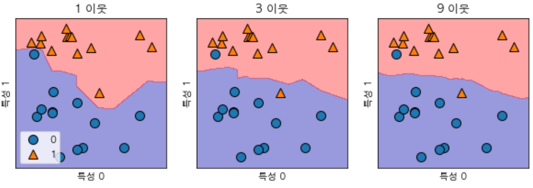
- 이웃 하나를 선택했을 때는 결정 경계가 훈련 데이터에 가깝게 따라가고 있다.
- 이웃의 수를 늘릴 수록 결정경계는 더 부드러워진다.(부드러운 경계는 단순한 모델을 의미)
- 이웃을 적게 사용하면 모델의 복잡도가 높아지고 많이 사용허면 복잡도는 낮아진다.
- 훈련 데이터 전체 개수를 이웃의 수로 지정하는 극단적인 경우에는 모든 테스트 포인트가 같은 이웃(모든 훈련 데이터)을 가지게 되므로 테스트 포인트에 대한 예측은 모두 같은 값이 된다.(훈련 세트에서 가장 많은 데이터 포인트를 가진 클래스가 예측값이 된다.)
정리
- 최근접 이웃의 수가 하나일 때는 훈련 데이터에 대한 예측이 완벽
- 하지만 이웃의 수가 늘어나면 모델은 단순해지고 훈련 데이터의 정확도는 줄어든다.
- 이웃을 하나 사용한 테스트 셋의 정확도는 이웃을 많이 사용했을 때보다 낮다.
k-최근접 이웃 회귀
- k-최근접 이웃 알고리즘은 회귀 분석에도 쓰인다.
- wave 데이터셋을 이용해서 이웃이 하나인 최근접 이웃을 사용
- x축에 세 개의 테스트 데이터를 흐린 별 모양으로 표시
- 최근접 이웃을 한 개만 이용할 때 예축은 그냥 가장 가까운 이웃의 타깃 값
mglearn.plots.plot_knn_regression(n_neighbors=1)
.png)
mglearn.plots.plot_knn_regression(n_neighbors=3)
.png)
- 여러 개의 최근접 이웃을 사용할 땐 이웃 간의 평균이 예측된다.
from sklearn.neighbors import KNeighborsRegressor

X, y = mglearn.datasets.make_wave(n_samples=40)
X_train, X_test, y_train, y_test= train_test_split(X, y, random_state=0)

reg = KNeighborsRegressor(n_neighbors=3)
reg.fit(X_train, y_train)
KNeighborsRegressor(algorithm='auto', leaf_size=30, metric='minkowski',
metric_params=None, n_jobs=None, n_neighbors=3, p=2, weights='uniform')
- 테스트 셋에 대한 예측
print('테스트 셋 예측 : \n {}'.format(reg.predict(X_test)))
테스트 셋 예측 :
 [-0.05396539  0.35686046  1.13671923 -1.89415682 -1.13881398 -1.63113382
  0.35686046  0.91241374 -0.44680446 -1.13881398]
- score로 모델 평가
- 이 메서드는 회귀일 땐 R^2의 값을 반환한다.
- 결정계수라고도 하는 R^2 값은 회귀 모델에서 예측의 적합도를 0과 1 사이의 평균으로 계산한 것
- 1은 예측이 완벽한 경우이고, 0은 훈련 셋의 출력값인 y_train의 평균으로만 예측하는 모델의 경우
print('테스트 셋 R^2: {:.2f}'.format(reg.score(X_test, y_test)))
테스트 셋 R^2: 0.83
KNeighborsRegressor 분석
- -3과 3 사이에 1,000개의 데이터포인트를 만든다.
- 1,3,9 이웃을 사용한 예측을 한다.
fig, axes = plt.subplots(1, 3, figsize=(15,4))
line = np.linspace(-3, 3, 1000).reshape(-1,1)
for n_neighbors, ax in zip([1,3,9], axes):
    reg = KNeighborsRegressor(n_neighbors=n_neighbors)
    reg.fit(X_train, y_train)
    ax.plot(line, reg.predict(line))
    ax.plot(X_train, y_train, '^', c=mglearn.cm2(0), markersize=8)
    ax.plot(X_test, y_test, 'v', c=mglearn.cm2(1), markersize=8)

    ax.set_title(
      "{} 이웃의 훈련 스코어:{:.2f} 테스트 스코어: {:.2f}".format(
          n_neighbors, reg.score(X_train, y_train),
          reg.score(X_test, y_test)))
    ax.set_xlabel('특성')
    ax.set_ylabel('타깃')

axes[0].legend(['모델 예측','훈련 데이터/타깃','테스트 데이터/타깃'], loc='best')
.png)
- 위의 그림에서 볼 수 있듯이 이웃을 하나만 사용할 때는 훈련 세트의 각 데이터 포인트가 예측에 주는 영향이 커서 예측값이 훈련 데이터 포인트를 모두 지나간다.
- 이는 매우 불안정한 예측을 만들어낸다.
- 이웃을 많이 사용하면 훈련 데이터에는 잘 안맞을 수 있지만 더 안정된 예측을 얻게된다.
장단점과 매개변수
- KNeighbors 분류기에 중요한 매개변수는 2개(데이터 포인트 사이의 거리를 재는 방법, 이웃의 수)
- k-NN의 장점은 이해하기 매우 쉬운 모델이라는 점
- 많이 조정하지 않아도 자주 좋은 성능을 발휘한다.
- 최근접 이웃 모델은 매우 빠르게 만들 수 있지만, 훈련셋이 매우 크면 예측이 느려진다.(특성의 수나 샘플의 수가 클 경우)
- k-NN 알고리즘을 사용할 땐 데이터를 전처리하는 과정이 중요.
- 수백 개 이상의 많은 특성을 가진 데이터셋에는 잘 작동하지 않고, 특성값이 대부분이 0인 데이터셋은 잘 작동하지 않는다.